
Formula for calculating dose rates from gamma emitting radioactive materials
Published: Mar 01, 2024
Source: Ionactive Radiation Protection Resource (Mark Ramsay, RPA)
Updated July2025
[Update July 2025: In addition to all the resource presented below, you may also find the following new resource interesting: Radioactivity to Dose Rate Calculator (with shielding and dose rate ratio options). ]
There are a number of formulae available for calculating gamma dose rates from radioactive material. Since the internet now has so much data available online, using a formula is probably consigned to academic interest. As long as you know the data is reliable (and seek Radiation Protection Adviser advice if required), then you will probably find using specific gamma ray constants of more use. Just try googling 'gamma ray constant Cs-137' and you will see what we mean! That said, you need to be really careful what you choose to use, you will sometimes find quite different values if you search for them.
In addition you should be careful what the result you search for really means. For example, is it in micro Gy/h or micro Sv/h? Is the result expressed as a dose rate in air, or a dose rate in tissue (or other substance)? Is the result expressed as an absorbed dose rate or ambient dose rate equivalent? Often the numerical value you seek may be about right, but are you sure how this is really being expressed (and does it actually matter?).
We did an internet search for Cs-137 which revealed the following results (we have converted all to SI units and scaled so they are directly comparable).
- 1156 micro Sv/h per GBq at 30 cm (search result 1)
- 848 micro Sv/h per GBq at 30 cm (search result 2, online calculator)
- 1146 micro Sv/h per GBq at 30 cm (search result 3)
Why the difference? Part of the difference is down to the derivation of the gamma ray constant and the dose unit it is quoted in (as noted above).
There is a temptation (and we did this above to make the point) to convert units without thinking too hard what they actually mean. For example, if you find an older resource in non SI units, is the value expressed in mR/h, mrad/hour or mrem/h?
In the first example above. according to the web page we landed on, our first result should actually read 1156 micro Gy/ h (this being derived from the data which was actually reported as 115.6 mR/hour (the R being the roentgen!). Without more thought (this was deliberate) we just multiplied mR by 10 and settled on the units of micro Sv/h. Is is this wrong? Does it matter?
A simple rule of thumb
Here is the rule of thumb formula (D=ME/6r2), it is something Mark Ramsay came across at the beginning of his career in radiation protection. It was in the book 'Introduction to Radiation Protection' by Alan Martin et al and was probably read about 1986. A link to the latest edition of this book can be found here: An Introduction to Radiation Protection Paperback (opens in a new window). We have no idea if the expression below features in the latest edition.
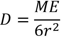
In this expression
D = Dose rate in (micro Sv/h)
M = Activity in MBq
E = Gamma energy in MeV
r = distance from the source in m
[Note: later in this resource Dr Chris Robbins will build this from first principles and M is replaced by A (since A more clearly denotes Activity].
The deceptively simple factor '6' actually ties up a load of variables converting activity (Bq) to disintegrations per second, eV to joules, joules per kg to Gy, Gy to Sv, seconds to hours, and accounting for an average (μen/ρ)airor (μen/ρ)tissue which is the mass energy absorption coefficient for material, and so on. The end result is an expression that sometimes works for the energy range of about 0.1 MeV up to 2 MeV (but see later below). The best way to think of D (micro Sv/h) is what you might expect to measure from an unshielded source using a typical workplace radiation monitor (which are normally tissue equivalent).
Using this rule of thumb with Cs-137
Let us use the equation with Cs-137 since its gamma emission (from the decay product Ba-137m) is simple (one gamma ray line of interest).
D = Dose rate in (micro Sv/h) - this is what we want
M = Activity in MBq (1000 MBq ,since we want 1GBq to match the search results we obtained earlier)
E = Gamma energy in MeV (0.662 MeV, obtained from any data book)
r = distance from the source in m (0.3 m to match the search results we obtained above).
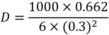
We see that D = 1226 micro Sv/h. A little higher than the above search results, but pretty close. (If you are not satisfied with 'pretty close' then please read to the end of this article).
A few things to note. Firstly, the expression as written only considers a single photon emission energy - such as with Cs-137. How about something a little more complicated.
Using this rule of thumb with Fe-59
Consider using the same expression with Fe-59. Looking in data tables we will find the following gamma energies with their emission probability:
1.292 MeV (43.2%)
1.099 MeV (56.5%)
0.192 MeV (3.1%)
0.143 MeV (1.0%)
We might want to leave out the bottom lower energy gammas as their emission probability is low (but as Chris Robbins will show later, this is not always a valid decision when you start to consider energy absorption) .
Considering E in the above equation, we now have the following:
E=(1.292 * 0.432)+(1.099*0.565)+(0.192*0.031)+(0.143*0.01) =1.19
Using exactly the same expression as above, but replacing (E) 0.662 (Cs-137) with 1.19 (Fe-59) we find that D is 2204 micro Sv/h.
Remember that the only difference is emission energy probability at each energy, the activity (M) is still 1 GBq (1000 MBq) and distance r is still 30 cm (0.3 m).
Now that we know how the above expression works, and it appears to provide reasonable values for Cs-137 in line with the literature, intuitively our value for Fe-59 (2204 micro Sv/h) should be about right.
- 1710 micro Sv/h per GBq at 30 cm (search result 1, online calculator)
- 1985 micro Sv/h GBq at 30 cm (search result 2)
Our value is a little higher than data obtained from a quick search online, but its still the right order of magnitude. The differences are fully explained later in this article.
As with all our rules of thumb resource, use carefully and contact a Radiation Protection Adviser (RPA) if unsure.
Additional thoughts on this rule of thumb
If you have made it down to here you may well just be curious, or perhaps you are not so happy with 'pretty close' or 'right order of magnitude'?
Use of energy probability. This is a lesson in not making assumptions. You will note above we explained how to deal with the energy (E) and emission probabilities for Fe-59. Well for Cs-137 we just made an assumption that its single 0.662 MeV gamma ray (actually from Ba-137m), was emitted with 100% probability. This is wrong, its actually 85.1% (Ref: NNDC). If we apply this emission probability to our calculated value of 1226 micro Sv/h for the Cs-137 (i.e. 0.662 MeV * 0.851) we find the dose rate reported is now 1051 micro Sv/h using the activity and distance as before. It might be that others have also incorrectly set the emission probability for Cs-137 to 100%?
Use of a generic single average (μen/ρ) (mass energy absorption coefficient). By 'use' we mean built into the above expression (tied up in the '6'). As you will see shortly below, the "6" in the above expression might be nearer "7". If we correct our 1051 micro Sv/h noted above, using "7" rather than "6" we find a dose rate of 900 micro Sv/h. This is much nearer some of our more reliable library values for Cs-137.
What is clear to see is that this rule of thumb does a reasonable job but has some significant omissions (probability of decay and energy specific absorption coefficients), and these will be particularly evident for radionuclides with many gamma emissions of low energy.
Do you want to take this further?
You should do! Understanding how a rule of thumb is put together, and where it should not be used (unless appropriately modified) is extremely important. So let Dr Chris Robbins of Grallator take it from here. Take it away Chris!
A "rule of thumb" for estimating the dose rate
Dr Chris Robbins, Grallator
[Ionactive note: as detailed earlier, in the analysis which follows A (activity) has replaced M as used in the formula above so far discussed].
Consider a point source of \(\gamma\)-rays which produces monochromatic photons of energy \(E\) MeV. Further, assume that each decay produces only one photon, and that the activity of the source is \(A\) MBq, i.e. \(A\) million decays per second \(\Rightarrow\) \(A\) million photons per second. We want to estimate the dose rate to a person in \(\mu Gy hr^{-1}\) at a distance \(r\) metres from the source, \(D_{\mu Gy hr^{-1}} (r) \).

Recall the definition of the gray (Gy) as a dose unit is
\(\qquad\)1 gray is the absorption of 1 joule or energy by 1 kilogram of matter.
The dose rate from this is how many joules of energy are absorbed per unit time per kilogram of matter. Note, the final expression will be in \(\mu\) joules per unit time per kilogram of matter.
Calculating the power
The total energy released per second (the power) in \({MeV \cdot s^{-1}}\), \(P_{MeV \cdot s^{-1}}\), is given by the energy per photon multiplied by the number of photons produced per second, i.e.
\[P_{MeV \cdot s^{-1}} = AE\times 10^6\]
where the \(\times 10^6\) takes account of the statement that the production rate is given in MBq.
The dose rate we are calculating uses units of \(\mu J\) for energy and hours for time. The above power is converted to these units by noting that
\(\qquad 1\,J = 1.6\times 10^{-19}\, eV = 1.6\times 10^{-13}\, MeV\)
\(\qquad 1\,hr = 60\, s/min \times 60\, mins/hr = 3.6\times 10^{3}\, s\)
So that \[P_{J \cdot hr^{-1}} = AE\times 10^6 \times 1.6\times 10^{-13} \times 3.6\times 10^{3} = 5.76AE\times 10^{-4}\] Noting that \( 1\,J = 10^{6}\,\mu J \), the above is given in terms of \(\mu J hr^{-1}\) as \[P_{\mu J \cdot hr^{-1}} = 5.76AE\times 10^{-4} \times 10^6 = 5.76AE\times 10^{2} = 576AE\]
Calculating the power density per unit area
At a distance \(r\) from the source, the energy released is spread over the surface of a sphere of radius \(r\), which has an area of \(4 \pi r^2\). The power per unit area at a distance \(r\) is therefore given by \[P_{\mu J \cdot hr^{-1} \cdot m^{-2}} = \frac{576AE}{4\pi r^2} = \frac{144AE}{\pi r^2} \] This is just the inverse square law.
What happens on the way to the measuring point?
While travelling from the source to the measuring point a distance \(r\) m away, the \(\gamma\) photons can be absorbed by the air. There is a fixed probability of absorption per unit distance travelled so the attenuation resulting from travelling a distance \(r\) in the air is of the form \[ I = I_0 e^{-\mu_a r}\] where
\(\quad\) \(I_0\) \(\quad\) is the initial photon intensity
\(\quad\) \(I\) \(\quad\) is the photon intensity after travelling a distance \(r\)
\(\quad\) \(\mu_a\) \(\quad\) is the linear attenuation coefficient for air, units m\(^{-1}\)
The dimensionless quantity \(e^{-\mu_a r} \equiv \mathrm {exp} (-\mu_a r) \) is the attenuation factor; it gives the fraction of the initial photons which travel the distance \(r\) without being absorbed.
An alternative form of the above is to use the mass energy attenuation coefficient, which is the linear attenuation coefficient normalised to the density of the material, air in this instance. The attenuation factor in this case is given by the expression \[ f_a = \mathrm {exp} \left(-\left(\frac{\mu_a}{\rho_a}\right) \rho_a r \right) \] Using the values for air of \( ({\mu_a}/{\rho_a}) = 2.676 \times 10^{-3}\, m^2 kg^{-1}\) and \(\rho=1.293 \, kgm^{-3}\) gives \(f_a = \mathrm {exp} \left(-3.46 \times 10^{-3} r \right) \). For a distance \(r=10\) m, the attenuation factor is \(f_a = 0.966\), i.e. there is very little absorption. In the approximation that is being derived we will ignore absorption in air under the assumption that the dose rate is being approximated "close" to the source.
Energy absorption rate at measuring point
At the measuring point we wish to calculate the energy absorbed per unit time per kg of matter (air, tissue, etc.). The attenuation factor for travelling through air has been given above. For travelling a distance \(x\) m through arbitrary matter the attenuation factor is \[ f_m = \mathrm {exp} \left(-\left(\frac{\mu_m}{\rho_m}\right) \rho_m x \right) \] As \(f_m\) gives the fraction of photons that pass through a distance \(x\) without being absorbed, then \(1-f_m\) must give the fraction that are absorbed over a distance \(x\). Applying this to the power density per unit area gives the energy absorption per unit area per unit time for matter thickness \(x\) of \[ \begin{align} P_{\mu J \cdot hr^{-1} \cdot m^{-3}} &= \frac{144AE}{\pi r^2 } \left(1- \mathrm {exp} \left(-\left(\frac{\mu_m}{\rho_m}\right) \rho_m x \right) \right) \end{align} \] Note, the attenuation factor may be found to be nearly one, however, as we are interested in the energy absorption rate we do cannot ignore absorption as we did for air as this would result in zero dose!
Simplifying things
The expression \(\mathrm{exp}(z) \) can be written as the Maclaurin series expansion \[ \mathrm{exp}(z) = 1+z+\frac{z^2}{2!}+\frac{z^3}{3!}+\cdots \] For the case where \(z\) is small \( \mathrm{exp}(z) \approx 1+z \). In our problem we wish to approximate \( \mathrm{exp}(-z)\) which is simply given by \( \mathrm{exp}(-z) \approx 1-z \). Using this approximation \[ \begin{align} \left(1- \mathrm {exp} \left(-\left(\frac{\mu_m}{\rho_m}\right) \rho_m x \right) \right) &\approx \left(1-\left( 1 - \left(\frac{\mu_m}{\rho_m}\right) \rho_m x \right) \right) \\ \\ &= \left(\frac{\mu_m}{\rho_m}\right) \rho_m x \end{align} \] Using this approximation gives \[ P_{\mu J \cdot hr^{-1} \cdot m^{-3}} = \frac{144AE}{\pi r^2 } \left(\frac{\mu_m}{\rho_m}\right) \rho_m x \] Reminder, this is valid if \(\left(\frac{\mu_m}{\rho_m}\right) \rho_m x \) is small.
What value of \(x\) to use?
The dose rate approximation we want is in \(\mu Gy hr^{-1}\), so, from the definition of a Gy, the value of \(x\) should be chosen to give 1 kg of matter. Using the relationship that \(\rho = \frac{mass}{volume}\), the volume of matter required to give 1 kg is \(V_m = \frac{1}{\rho_m} \, m^3\). The power density above is given per unit area, so the value of \(x\) required as a depth over this unit area to give a volume of \(\frac{1}{\rho_m} \, m^3\) is approximately \(\frac{1}{\rho_m} \, m\), if this value is small enough that the surface areas of the upper and lower volume element faces are approximately equal. Using this gives an expression for the absorption factor as \[ \left(\frac{\mu_m}{\rho_m}\right) \rho_m x = \left(\frac{\mu_m}{\rho_m}\right) \rho_m \frac{1}{\rho_m} = \left(\frac{\mu_m}{\rho_m}\right) \] The energy absorption per unit area per unit time for 1 kg of matter is then given by \[ D_{\mu Gy hr^{-1}} \equiv P_{\mu J \cdot hr^{-1} \cdot kg^{-1}} = \frac{144AE}{\pi r^2 } \left(\frac{\mu_m}{\rho_m}\right) \] This is the dose rate expression we are seeking.
Using values of \( ({\mu_m}/{\rho_m}) = 3.40 \times 10^{-3}\, m^2 kg^{-1}\) and \(\rho=1000 \, kgm^{-3}\) as 'typical' values for tissue gives \(x = \frac{1}{1000} \,m\) and an absorption factor of \[ \left(\frac{\mu_m}{\rho_m}\right) = 3.40 \times 10^{-3} \] This value is small and so the approximation to remove the exponential function is valid. Also, the value of \(x\) is small, so the approximation of the volume being a small regular prism with a base of unit area is also valid.
Note, for air the expression \[ \begin{align} \left(\frac{\mu_m}{\rho_m}\right) \rho_m x = \left(\frac{\mu_m}{\rho_m}\right) \rho_m \frac{1}{\rho_m} &= 2.676 \times 10^{-3} \times 1.293 \times \frac{1}{1.293} \\ \\ &= 2.676\times 10^{-3} \end{align} \] is also small, however \(x=\frac{1}{1.293}\) is not small so inverse square effects could become important. In this case, the correct volume element should be a frustum of a pyramid or a cone, and the value of \(x\) will be reduced to account for this. This is not considered here, so the dose rate derived here will apply more correctly to relatively dense matter such as tissue.
The dose rate rule of thumb expression
Using a fixed tissue absorption factor of \( ({\mu_m}/{\rho_m}) = 3.40 \times 10^{-3}\), the final expression for the dose rate rule of thumb in units of \(\mu Gy hr^{-1}\) is \[ \begin{align} D_{\mu Gy hr^{-1}} &= \frac{144AE}{\pi r^2 } \times 3.40 \times 10^{-3} \\ \\ &=\frac{306AE}{625 \pi r^2 } \\ \\ \end{align} \] A further simplification can be made by taking the gross approximation that \(\frac{306}{625 \pi} \approx \frac{1}{6} \) to the nearest simple fraction so that the rule of thumb dose rate becomes \[ \begin{align} D_{\mu Gy hr^{-1}} &= \frac{AE}{6 r^2 } \end{align} \] For \(A\) in MBq, \(E\) in MeV and \(r\) in metres.
What happens if multiple photons with multiple energies are emitted?
It is not unusual for a \(\gamma\) source to produce a spectrum of photon energies. In this case, the energy should be averaged over all the photon energies possible through \[ E = \sum_i p_i E_i \] where \(p_i\) is the probability that a photon of energy \(E_i\) is released during the decay. In some cases the evaluation of the above can be quite involved and multiple photons can be released. For example, \(^{60}Co\) has two decay paths:
99.88% of decays give two \(\gamma\) photons of energy 1.1732 MeV and 1.3325 MeV respectively
0.12% of decays give one \(\gamma\) photon of energy 1.3325 MeV
In this case the total photon energy released per decay is
\[E = (0.9988 \times 1.1732) + (0.9988 \times 1.3325) + (0.0012 \times 1.3325) = 2.5043 MeV\]
Warning, this is only valid if \( ({\mu_m}/{\rho_m})\) is a fixed value for all photon energies, as in the above assumption!
Other units
The gray (Gy) is converted to sieverts (Sv) by multiplying by a quality weighting factor \(W_R\). For X-rays and \(\gamma\) rays \(W_R=1\) so the above dose rate in \(\mu Sv hr^{-1}\) is simply given by multiplying the dose rate in \(\mu Gy hr^{-1}\) by 1 to give \[ \begin{align} D_{\mu Sv hr^{-1}} &= \frac{AE}{6 r^2 } \end{align} \] For \(A\) in MBq, \(E\) in MeV and \(r\) in metres.
Does the rule of thumb work?
The rule of thumb expression has been derived using a number of assumptions and simplifications. By far the biggest of these are that a fixed value of the absorption factor, \( ({\mu_m}/{\rho_m}) = 3.40 \times 10^{-3}\) is used and \(\frac{306}{625 \pi} \approx \frac{1}{6} \). For the latter, \(\frac{306}{625 \pi} = \frac{1}{6.41665\, \dots} \) so even if the absorption factor is appropriate, the rule of thumb expression will tend to over-predict values by about 7%.
It is also important to note that in reality the absorption factor varies with photon energy and the matter that is absorbing it, so the rule of thumb is only technically valid for a source with an energy release being absorbed by matter with an absorption coefficient of \( ({\mu_m}/{\rho_m}) = 3.40 \times 10^{-3}\). In fact this value is slightly high for most tissues but reasonably flat over an energy range of 0.05 to 2 MeV. For generic values you should revert to the full expression \[ D_{\mu Gy hr^{-1}} = \frac{144AE}{\pi r^2 } \left(\frac{\mu_m}{\rho_m}\right) \] For lower values of \( ({\mu_m}/{\rho_m})\), the above could approximate to \(D_{\mu Sv hr^{-1}} = \frac{AE}{7 r^2 }\) or \(D_{\mu Sv hr^{-1}} = \frac{AE}{8 r^2 }\), etc.; the actual best rule of thumb depends on circumstances.
When a number of photons can be released, as in the \(^{60}Co\) example above, the total dose rate should be calculated as the sum of the dose rates of each photon. Do not use the energy averaging above. \[ \begin{align} D_{\mu Gy hr^{-1}} &= \sum\limits_i p_i\frac{144AE_i}{\pi r^2 } \left(\frac{\mu_m}{\rho_m}\right)\bigg |_{E_i} \\ \\ &= \frac{144A}{\pi r^2 } \sum\limits_i p_i E_i \left(\frac{\mu_m}{\rho_m}\right)\bigg |_{E_i} \end{align} \] where \(p_i\) is as before and \( ({\mu_m}/{\rho_m}) | _{E_i} \) is the value of \( ({\mu_m}/{\rho_m})\) for a photon of energy \(E_i\).
For the \(^{60}Co\) example used above the following energies, probabilities and energy absorption coefficients for soft tissue are used.
| i | \(E_i \,\,(MeV) \) | \(p_i\) | \( (\mu_m / \rho_m)\,\, (m^2/kg) \) | \( p_i E_i (\mu_m / \rho_m) |_{E_i} \) |
| 1 | 1.1732 | 0.9988 | \(2.9760 \times 10^{-3}\) | \(3.4873 \times 10^{-3}\) |
| 2 | 1.3325 | 0.9988 | \(2.9047 \times 10^{-3}\) | \(3.8659 \times 10^{-3}\) |
| 3 | 1.3325 | 0.0012 | \(2.9047 \times 10^{-3}\) | \(4.6446 \times 10^{-6}\) |
\[\begin{align}D_{\mu Gy hr^{-1}} &= \frac{144A}{\pi r^2 } \sum\limits_i p_i E_i \left(\frac{\mu_m}{\rho_m}\right)\bigg |_{E_i} \\ \\&= \frac{144A}{\pi r^2 } \left( 3.4873 \times 10^{-3} + 3.8659 \times 10^{-3} + 4.6446 \times 10^{-6} \right) \\ \\&= \frac{144A}{\pi r^2 } \times 7.3578\times 10^{-3} \\ \\&\approx \frac{A}{2.83 r^2 }\end{align}\]
What happens if you work backwards from the above result to get an expression of the form \[ \begin{align} D_{\mu Gy hr^{-1}} &= \frac{AE}{N r^2 } \end{align} \] for an appropriate total energy \(E\) and integer \(N\)? The working above has calculated a single value for the total energy E for \(^{60}Co\) as \(E=2.5043 MeV\). Multiplying the actual value top and bottom by this value for \(E\) (keeping the symbol on the top and substituting the value on the bottom) gives \[ \begin{align} D_{\mu Gy hr^{-1}} &= \frac{A}{2.83 r^2 } \times \frac{E}{E} \\ \\ &=\frac{A}{2.83 r^2 } \times \frac{E}{2.5043} \\ \\ &\approx \frac{AE}{7 r^2 } \end{align} \] So, nearly the rule of thumb, but with a slightly larger denominator.
Can low energy photons be ignored?
From the expression \[ \begin{align} D_{\mu Gy hr^{-1}} &= \frac{144A}{\pi r^2 } \sum\limits_i p_i E_i \left(\frac{\mu_m}{\rho_m}\right)\bigg |_{E_i} \\ \\ \end{align} \] it is noted that the contribution to the total dose rate from a photon of energy \(E_i\) is proportional to \( p_i E_i (\mu_m / \rho_m) |_{E_i} \). The example above is for a case where all the possible photons are of broadly similar energy, with similar energy absorption coefficients, so contributions are dominated by the first two photons in the list. However, there are sources, such as \(^{192}Ir\) that produce \(\gamma\) photons over a wide range of energies from 9 keV to 612.5 keV. It may be tempting to ignore low energy photons in the calculation, but this should be done with caution as, although a 9 keV photon has about 1/68 the energy of a 612.5 keV photon, its energy absorption coefficient is several orders of magnitude higher, as shown in the following graph.

The table below gives values and dose rate contributions from all the possible photon emissions of \(^{192}Ir\). Note, the derived values below may show rounding effects due to the source values having more decimal places than displayed.
| i | \(E_i \,\,(MeV) \) | \(p_i\) | \( (\mu_m / \rho_m)\,\, (m^2/kg) \) | \( p_i E_i (\mu_m / \rho_m) |_{E_i} \) | Dose rate contribution |
| 1 | 0.0090 | \(1.470 \times 10^{-2}\) | \(6.9051 \times 10^{-1}\) | \(9.1355 \times 10^{-5}\) | 3.13% |
| 2 | 0.0094 | \(4.000 \times 10^{-2}\) | \(5.9586 \times 10^{-1}\) | \(2.2500 \times 10^{-4}\) | 7.70% |
| 3 | 0.0615 | \(1.170 \times 10^{-2}\) | \(3.2031 \times 10^{-3}\) | \(2.3044 \times 10^{-6}\) | 0.08% |
| 4 | 0.0630 | \(2.020 \times 10^{-2}\) | \(3.1440 \times 10^{-3}\) | \(4.0010 \times 10^{-6}\) | 0.14% |
| 5 | 0.0651 | \(2.630 \times 10^{-2}\) | \(3.0651 \times 10^{-3}\) | \(5.2494 \times 10^{-6}\) | 0.18% |
| 6 | 0.0668 | \(4.520 \times 10^{-2}\) | \(3.0047 \times 10^{-3}\) | \(9.0762 \times 10^{-6}\) | 0.31% |
| 7 | 0.0714 | \(8.700 \times 10^{-3}\) | \(2.8558 \times 10^{-3}\) | \(1.7740 \times 10^{-6}\) | 0.06% |
| 8 | 0.0757 | \(1.970 \times 10^{-2}\) | \(2.7304 \times 10^{-3}\) | \(4.0719 \times 10^{-6}\) | 0.14% |
| 9 | 0.1363 | \(1.810 \times 10^{-3}\) | \(2.6965 \times 10^{-3}\) | \(6.6544 \times 10^{-7}\) | 0.02% |
| 10 | 0.2013 | \(4.660 \times 10^{-3}\) | \(2.9454 \times 10^{-3}\) | \(2.7631 \times 10^{-6}\) | 0.09% |
| 11 | 0.2058 | \(3.290 \times 10^{-2}\) | \(2.9571 \times 10^{-3}\) | \(2.0021 \times 10^{-5}\) | 0.69% |
| 12 | 0.2833 | \(2.610 \times 10^{-3}\) | \(3.1316 \times 10^{-3}\) | \(2.3152 \times 10^{-6}\) | 0.08% |
| 13 | 0.2960 | \(2.896 \times 10^{-1}\) | \(3.1563 \times 10^{-3}\) | \(2.7052 \times 10^{-4}\) | 9.26% |
| 14 | 0.3085 | \(2.967 \times 10^{-1}\) | \(3.1721 \times 10^{-3}\) | \(2.9030 \times 10^{-4}\) | 9.94% |
| 15 | 0.3165 | \(8.284 \times 10^{-1}\) | \(3.1796 \times 10^{-3}\) | \(8.3367 \times 10^{-4}\) | 28.54% |
| 16 | 0.3745 | \(7.290 \times 10^{-3}\) | \(3.2293 \times 10^{-3}\) | \(8.8159 \times 10^{-6}\) | 0.30% |
| 17 | 0.4165 | \(6.620 \times 10^{-3}\) | \(3.2526 \times 10^{-3}\) | \(8.9673 \times 10^{-6}\) | 0.31% |
| 18 | 0.4681 | \(4.780 \times 10^{-1}\) | \(3.2631 \times 10^{-3}\) | \(7.3006 \times 10^{-4}\) | 25.00% |
| 19 | 0.4846 | \(3.160 \times 10^{-2}\) | \(3.2662 \times 10^{-3}\) | \(5.0012 \times 10^{-5}\) | 1.71% |
| 20 | 0.4891 | \(3.970 \times 10^{-3}\) | \(3.2670 \times 10^{-3}\) | \(6.3431 \times 10^{-6}\) | 0.22% |
| 21 | 0.5886 | \(4.520 \times 10^{-2}\) | \(3.2556 \times 10^{-3}\) | \(8.6609 \times 10^{-5}\) | 2.97% |
| 22 | 0.6044 | \(8.180 \times 10^{-2}\) | \(3.2520 \times 10^{-3}\) | \(1.6078 \times 10^{-4}\) | 5.50% |
| 23 | 0.6125 | \(5.330 \times 10^{-2}\) | \(3.2484 \times 10^{-3}\) | \(1.0604 \times 10^{-4}\) | 3.63% |
The above table shows that the two lowest energy photons contribute more than 10% to the total dose rate because they are far more easily absorbed. In fact the two lowest energy photons contribute more to the total dose rate than the two highest energy photons, even though there are more than twice as many of the two highest energy photons produced as there are the two lowest energy photons.
Dr Chris Collins can be contacted at Grallator (opens in a new window).
How about an interactive demonstration?
Have a play with this radiation protection widget, the first to go live on the Ionactive website.